A Nomograph for Artillery Range

Recent news surrounding the supply of North Korean “Koksan” self-propelled artillery pieces to Russia, as part of the ongoing Russo-Ukraine conflict, has sparked online debate regarding its performance characteristics, much of which was (and remains) unknown due to the boutique caliber this gun is chambered in.

While it remains my position that most of it amounted to internet sleuthing with no real basis in reality, this discourse highlighted the lack of accessible resources supporting analysis of artillery performance characteristics online: while existing online exterior ballistics applications like Big Gun Ballistics supports performing exterior ballistics calculations, the calculation is presented in a one-shot manner, not unlike the command line computer programs of old, and there is no provision for solving the reverse problem, or finding the gun parameters required for a given range.

Which brings us to the idea of constructing a nomograph, or nomogram. As a quick primer on nomgraphs (and as the WordPress software is marking these words out to be grammar mistakes as I was typing, I figured most of you probably need this), at the most basic level, nomographs represents a particular calculation, with the parameters laid out as points on (usually) two scales, and when a line is drawn over the two, the solution is found where the third scale is intersected.

The brilliance of the nomograph as it applies to this problem is that, with there being no preferred direction for the calculation to be ran in. The user can, as easily, start from the “solution” and work backward to find the value of one “parameter” given another. Therefore, if a nomographic representation of artillery range is constructed, the same nomograph can be used to shed light on the necessary condition for given range to be achieved.

As well, a nomograph is also desirable from a public outreach standpoint. Once constructed, they can be disseminated online as a single image or file, or printed out on to a piece of paper without loss of information or functionality. Ofcourse, this comes at the cost of limited practical accuracy, but for our purposes, this is less critical.

Then it only remains to lay out the principles, the math, crunch the numbers, and create the nomograph.

The Exterior Ballistics

To model the motion of a projectile in the exterior ballistic environment, we first need to model the atmosphere that it travels within.

Introducing the (Chinese) Standard Artillery Atmosphere, which, with the reference values of an ambient temperature of 288.15 K (or 15 °C), ambient pressure of 101.325kPa (or 750 mmHg), and a relative humidity of 50%, together with additional assumptions with the gun sited on the mean sea level, at a latitude of 45 degrees, shooting at a target at the same height. The range achieved with this incredibly specific set of conditions is the usual value that is quoted for older Chinese pieces (including those reverse engineered from the Soviet Union).

Given these reference conditions, the model gives the humidity corrected temperature $\tau$ ¹, with regard to height above ground, $h$ , in meters, as:

$\tau(h) = \begin{cases} 289.1 - 6.328\times 10^{-3} h & h \leq 9300 \text{m} \\ 230.2 - 6.328\times 10^{-3} (h-9300) + 1.172\times 10^{-6} (h-9300)^2 & h\leq 12000\text{m} \\ 221.7 & \text{otherwise} \\ \end{cases}$

The first linear segment characterizes a linear decrement in the troposphere, transitioning into a more gradual quadratic decrease in the substratosphere region, and holding the same in the stratosphere.

From this, the local density, $\rho$ , in kg/m³, can be estimated from the pressure $p$ , in Pa, as:

$\rho(p, \tau) = \cfrac{p}{287 \tau}$

And the local sonic velocity $c$ , in m/s, as:

$c(\tau) = \sqrt{1.40 \cdot 287 \tau}$

Within this environment, the drag, $f_d$ acting upon a spin stabilized projectile can be modeled as a function of the dynamic pressure impinging upon it, $\frac{1}{2} \rho v^2$ , and the cross section, $S$ , with the fairly well known equation:

$f_d = \frac{1}{2} \rho v^2 C_d S$

The relationship factor, $C_d$ , is often referred to as the drag coefficient, or the coefficient of drag. For spin stabilized, roughly spitzer shaped projectiles, it is more appropriate to think of it not as a set value, but as a function, chiefly of the local Mach number, $M = v/c$ . However, obtaining this function dependence $C_d(M)$ before doppler velocimeter was far from trivial. Consequently, the most practical approach that was settled upon, was to come up with some reference $C_d(M)$ function that is accurately determined for a reference projectile, and assign projectiles a shape factor, $i$ , that represent the ratio of drag experienced by this projectile to the reference value. These standardized reference functions are known as drag curves.

In the Soviet Union and in China, the most well known drag curve is that of the 1943 drag curve, which was originally in tabular form. Over the years, curve fits have been developed that produce a reasonable approximation while being much more convenient for computational uses. One such example is reproduced here, with a peak difference of less than 3% (in the transonic region):

$C_{d,43}(M) = \begin{cases} 0.157 & M < 0.79 \\ 0.260 & M > 3.95 \\ \cfrac{0.15494 - 0.38989 M^2 + 0.38100 M^4 - 0.23778 M^6 + 0.11412 M^8}{1 - 2.6458 M^2 + 2.7429 M^4 - 1.4990 M^6 + 0.47141 M^8} & \text{otherwise} \end{cases}$

With all of the above, the drag of a projectile may be rewritten in the form:

$f_d = \frac{1}{2} \rho(h, p) v^2 i_{43} C_{d,43}(v/c) S$

For ground artillery ranges, the Coriolis correction can be omitted (at least at the initial design stage), which reduce the problem to the numerical integration of the equation of motion describing projectile motion under drag and gravity, in 2 dimensions. This, when projected in an rotating reference frame, with the height ( $h$ ) axis along the earth’s radius, and the range ( $r$ ) axis along the circumference, yields the following system of equations:

$\begin{cases} \cfrac{d v_{r}}{dt} = -\cfrac{1}{2} \rho v v_{r} i_{43} C_{d,43}(v/c) \cfrac{S}{m} - \cfrac{v_r v_h}{R+h} \\ \cfrac{d v_{h}}{dt} = -\cfrac{1}{2} \rho v v_{h} i_{43} C_{d,43}(v/c) \cfrac{S}{m} + \cfrac{v_r^2}{R+h} - g \\ \cfrac{dr}{dt} = \cfrac{v_r}{1 + h/R} \\ \cfrac{dh}{dt} = v_h \\ \cfrac{dp}{dt} = -\rho g v_y \\ g = \cfrac{g_0}{(1+h/R)^2} \\ v = \sqrt{v_r^2+v_h^2} \end{cases}$

In which, $m$ denotes the mass of a projectile, $R$ denotes the distance between mean sea level and the center of the earth, and $g_0$ denotes the acceleration of gravity at the aforementioned mean sea level, reference value of 6356766 meters and 9.80665 m/s, respectively.

This concludes the familiar territory.

The Math and Programming

This series of equation is integrated numerically until impact to calculate the range of a projectile given its caliber, mass, shape factor, the initial velocity, and the elevation. For this work, I have elected to implement a Runge-Kutta 4(5)th order method, as is common practice. This yields a function $f(d, m, i_{43}, v, \theta) \to r$ .

As $d$ , $m$ and $i_{43}$ all only appear as a factor in the drag equation, it is convenient to further factor these into an “adjusted sectional density”, or $\frac{4m}{i_{43} \pi d^2} = \frac{m}{i_{43} S}$ without any loss in generality. The function is then reduced to $f(\frac{m}{i_{43} S}, v, \theta) \to r$ .

The effect of the various factors on the elevation to achieve optimal ground range is a bit complicated, as illustrated by the following figure.

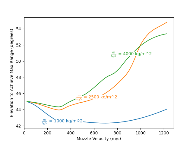
For projectiles at very low velocity, the drag experienced is very small, and consequently the optimal range trajectory is close to the vacuum solution, or launching at exactly 45 degrees. Then, as the effect of drag become significant with increasing velocity, which is more so for projectiles with a lower (adjusted) sectional density, the trajectory becomes increasingly asymmetric: the climb out to maximum range is much less steep than the descent to target, which incentivizes lower angles that better utilize this phase of flight.

The optimum range elevation stops decreasing as muzzle velocity goes transonic, and continues upward as the muzzle velocity goes supersonic. The driving concern for this regime is the transonic drag spike of the projectile, where the projectile experiences the most drag in relation to the dynamic pressure (in fact close to thrice as high as in the subsonic regime, and twice as high as in the deep supersonic regime). An increase of elevation at this point allows the projectile to quickly climb out of the densest part of the atmosphere, even at the cost of initial horizontal velocity, with the overall effect being net beneficial to achieving longer range.

Eventually, as the projectile’s velocity and range further increases, the optimal initial elevation slowly decreases again, due to the curvature of earth.

As a result of the complex interplay of these factors, the optimal elevation to achieve maximum ground range has to be found numerically. Let this optimal routine output the optimal range, $g(\frac{m}{i_{43} S}, v) = \max\limits_{\theta\in(0,\frac{\pi}{2})} f(\frac{m}{i_{43} S}, v, \theta) \to r_{opt}$ . I have checked to the best of my ability that function $f$ is uni-modal in the relevant parameter space. Assuming this being the case, a Gold-Section search with $\theta \in (0, \frac{\pi}{4})$ , and with all other parameters fixed, has been found to work well. This has been used to produce the previous figure.

One last issue to sort out: the function $g$ is the result of running a numerical optimization routine over a numerical integration routine. Due to the finite accuracy involved in each step, the resulting function by necessity has to be discrete, i.e. it is only smooth and continuous at an scale much larger than the accuracy of numerical integration and the allowable error in the numerical optimization routine. When the function is called with a small variation in input variable, the output can behave randomly if the variation is small enough. Functions with these characteristics are not well handled by the nomography module that I chose to rely on.

The solution I came up with is to perform a rough sampling of the parameter space, at a scale much larger than the accuracy and allowable error of the numerical routines. Then, a bi-variate spline interpolation is performed on the result.

This results in a “surrogate” function $g\prime \approx g$ . With some finesse, this can result in a fairly accurate approximation. The below figure illustrates one such fit, using only 10 samples along each axis, for the parameter space $v\in [500, 2000], \frac{m}{i_{43} S} \in [1000, 4000]$ . The surrogate function is accurate to within 1 percent of the true result in terms of range, accurate enough for our purpose.

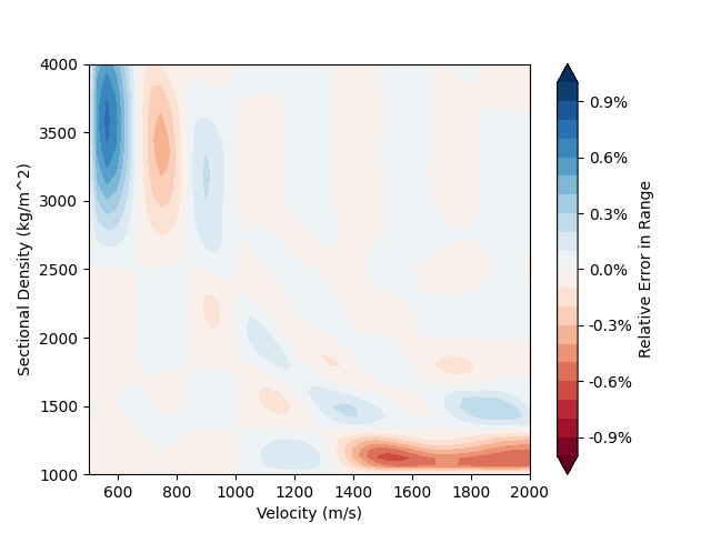
The drawback of this approach is that it appears difficult to find a fit that is accurate for both the subsonic and supersonic regime, as the function behaves rather differently.

This is not too inconvenient, as I had already anticipated the need for multiple nomographs. As an example, the range of a field gun may be as high as 30 or 40 kilometers, with a muzzle velocity as high as 1,000 m/s or more, while most mortars and infantry guns barely reach 10 kilometers, and is rarely supersonic. If these are plotted on the same graph, then all the mortar solutions would be cramped into a corner, and their range can only be read to a lesser accuracy. Producing separate graphs with each tailored to the performance regime of that category of weapon should increase the legibility and practical accuracy of the graphs.

The Nomograph

Finally, with all of the preparation done, the pyNomo package is used to generate the following nomographs, available to download as portable data files.

nomograph_of_artillery_ranges_(howitzer_and_field_guns)Download

nomograph_of_artillery_ranges_(mortars)Download

The howitzer and field guns nomograph is constructed from 500 m/s and up, with a range scale from 5 km up to 50 km. The mortar nomograph is constructed from 50 m/s up to 500 m/s, with a range scale from 0 to 15 km. This choice gives some headroom for exploring more the performance of pieces with more aggressive specifications, while retaining reasonable accuracy and legibility. A selection of pieces and their graphical solution has been plotted as convenient references.

Perfection is the enemy of progress, as they say. I fully expect to be tweaking these over the coming months, but I am happy enough with these as-is to share them with the internet at large.

For those interested, the corrected temperature $\tau$ is related to the measured tempreature $\tau =T/ (1-\frac{3 p_w}{8 p})$ , with $p$ and $p_w$ being the partial pressure of air and water vapour, respectively.
The influence of water vapour on exterior ballistics is to introduce a gas component with a lower index of specific heat, which slightly raises the sonic velocity and reduces the density of the mixture. This is conveniently expressed as a modification to the temperature. ↩︎

The Meandering of a Ballistics Oriented Mind